The Origin-Destination Matrix
In this section, we will be looking into the so-called origin-destination matrix, or the OD matrix. The OD matrix tells us the trip distribution between a pair of locations $(p, q)$. There are many representations of the OD matrix. It can be represented using a matrix, a network, or the generating process behind it.
The Matrix
The origin-destination matrix describes ${g_{pq}}$ for origin-destination pairs $pq\in P\bigotimes Q$.
We show an example using the international road freight data from Eurostats.1 The are many different representations of the origin-destination matrix. The data can be represented using tabular data. On the other hand, it is easier to interpret if we introduce some visualization elements. For example, we visualize the matrix using a heatmap where we color code the amount of goods transported in unit of million-tonne-kilometer.
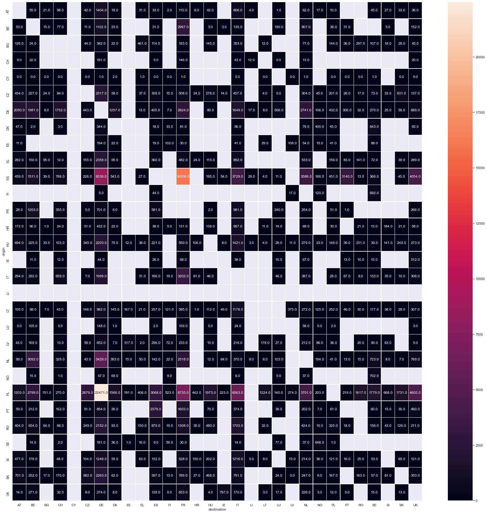
Visualization of goods loaded unloaded in Europe. The gray cells in the charts indicates missing data.
Alternatively, we can visualize this matrix using networks.
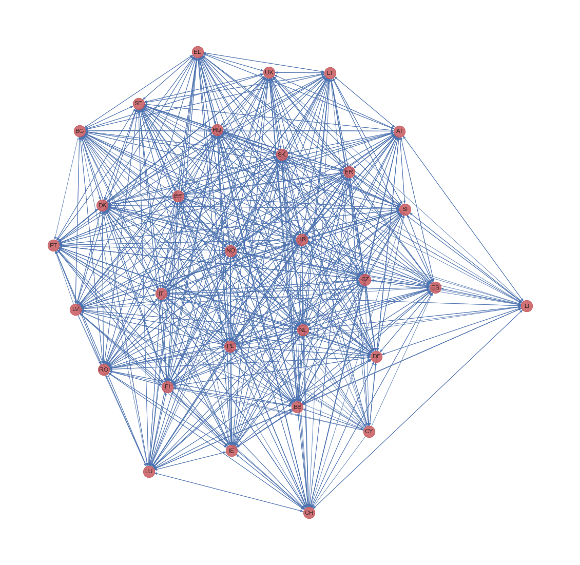
Visualization of goods loaded unloaded in Europe using networks. Some countries are less connected.
There are other visualizations of networks such as arc plots and circle plots. In the end, visualizations are just some of the representations of the matrix. A much more powerful representation is a way to describe the generating process of the origin-destination matrix. For example, we could represent the underlying generating process with a function. The function itself, could as well be a neural network if desired.
A Generating Process behind the Origin-Destination Matrix
Simply describing the data is not so satisfying. What is more powerful is to find or construct a simple model to describe the underlying generating process so it can be used to find causalities and predict the future. One of such models is the gravity model.
The gravity model is a simple distribution model where we assume the distribution is proportional to the two masses: the flow out of the origin and the flow into the destination. In this section, we will follow A. Peterson to demonstrate the basic ideas of this model2. The flow between origin $p$ and destination $q$ is assumed to be proportional to the multiplication of them, as the gravitational force between to massive objects,
$$ g_{pq} = k_{pq} o_p d_q f(\pi_{pq}), $$
where $\pi_{pq}$ is the travel impedance. We have
$$ o_p = \sum_q g_{pq} $$
and
$$ d_q = \sum_p g_{pq}. $$
The deterrence function $f(\pi_{pq})$ can have many different forms as long as it captures the factors of friction:
- polynomial: $\pi_{pq}^{-\beta}$,
- exponential: $e^{-\beta \pi_{pq}}$.
The coefficient $k_{pq}$ is also taking care of the fact that the dependency on the masses $o_p$ and $d_q$ and the deterrence can be different for different lanes.
Given the fact that the total flow out of $p$ is
$$ o_p = \sum_q g_{pq} = o_p\sum_q k_{pq} d_q f(\pi_{pq}), $$
we thus derive a simple identity
$$ \sum_q k_{pq} d_q f(\pi_{pq}) = 1. $$
Modal Split
The split of the loads between origin and destination can also be assigned to different modes, i.e., partitioning of the flow based on travel modes $g^k_{pq}$. In this section, we review a method called multinomial logit model introduced in A. Peterson (2007)2. We use the probability of modes $p_k$ to describe the split, i.e., $g_{pqk} = g_{pq}p_k$.
To partition the flow, a utility function $u_k$ of each mode $k$ is introduced. The utility function considers:
- Some attributes denoted by $h$, $h$ can be walking time, transport time, etc. All the attributes form a set $H$ where $h\in H$;
- Travel mode $k$;
- The measured value of attribute $h$ for travel mode $k$: $x_{hk}$;
- Weighting parameter $\alpha_h$.
The utility function has two major parts. The part of utility that can be modeled
$$ v_k = \sum_h \alpha_h x_{hk}, $$
as well as a part from the random effects. The actual utility may have some random effects $\epsilon_k$,
$$ u_k = v_k + \epsilon_k. $$
The multinomial logit model assumes the probability of the mode $k$ to be
$$ p_k = \frac{e^{\mu u_k}}{ \sum_k e^{\mu u_k} } = \frac{e^{\mu v_k} e^{\mu \epsilon_k}}{ \sum_k e^{\mu u_k} e^{\mu \epsilon_k} }. $$
The non-linearity leads to some problems. Different combination of modes leads to contradictory results.2 One solution to such problems is to come up with a fixed hierarchy model.
References
Eurostats is a good place to find datasets about Europe. For example, the provide a dataset on goods loaded in reporting country with illustrations of the data here. ↩︎
Peterson, A. (2007). The Origin–Destination Matrix Estimation Problem — Analysis and Computations. In Journal of Scientific and Industrial Research (Vol. 67). ↩︎ ↩︎ ↩︎
L M (0001). 'The Origin-Destination Matrix', The Flow, 01 April. Available at: https://flow.leima.is/road-freight/basics/origin-destination-matrix/.